Agent Cost ≠ App Cost: Why Traditional Ops/Cost Calculation Methods Do Not Apply to Agents
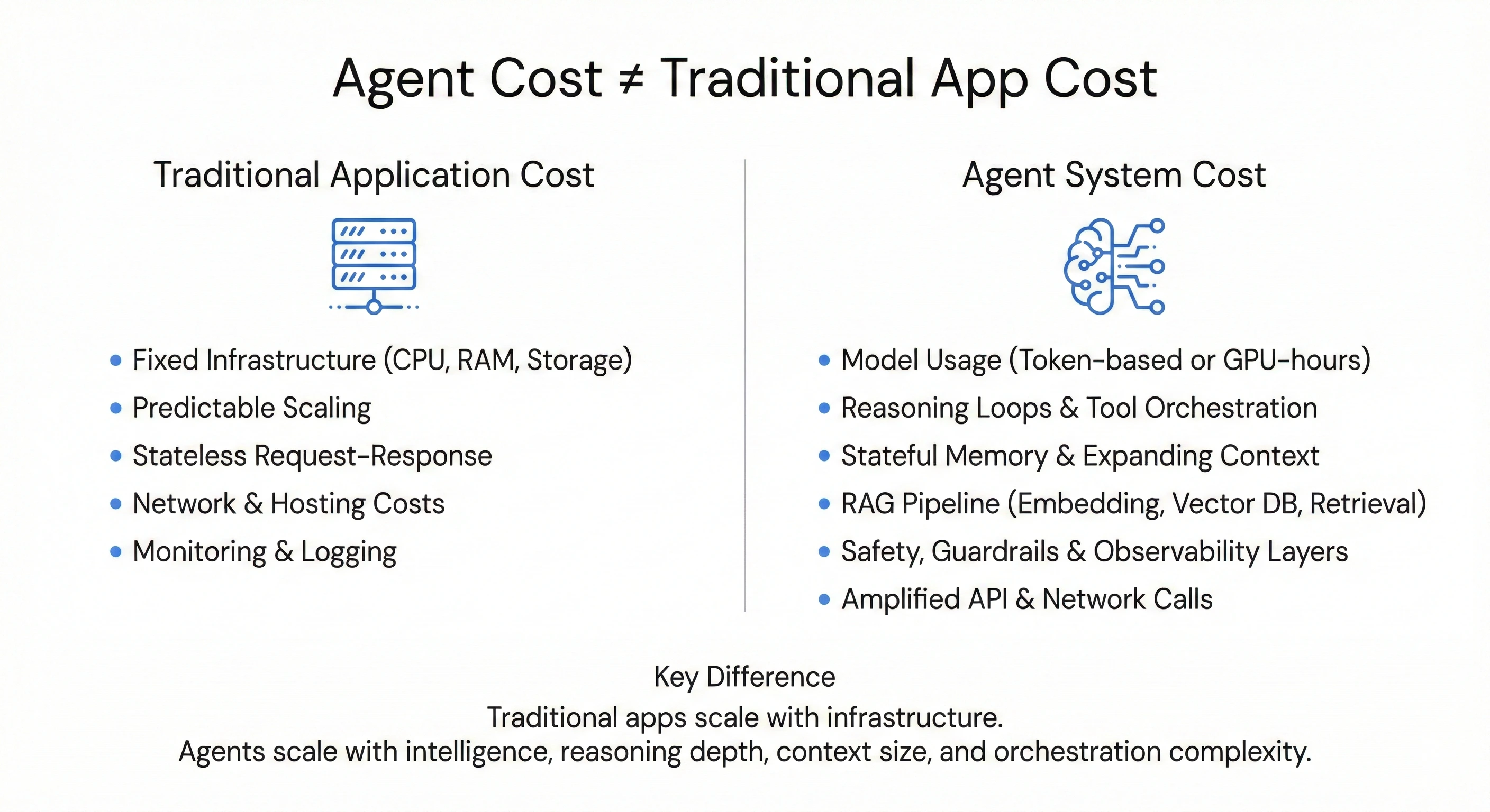
1. Additional Costs That Traditional Applications Do Not Have
- Model usage: This is usually the biggest cost. Instead of only paying for fixed infra like CPU/RAM/Disk, we now pay per token (when using APIs like OpenAI, Google Gemini, Anthropic, etc.) or per GPU-hours if we self-host open-source models. Every input prompt, every output, and even the reasoning tokens generated by the LLM are charged.
- Reasoning loops & Tool orchestration: In an agentic architecture, one query is not a simple linear request/response. It is a dynamic workflow: plan → reason → act → observe → refine. Every step in that loop — from LLM calls for reasoning to calling external tools/APIs — adds cost.
- Stateful memory & Context: Unlike traditional stateless systems, Agents need to maintain conversation state. Each turn has to rebuild context from previous history, which makes the prompt size grow over time. The longer the session, the larger the context. At the same time, RAG and Vector DB are almost mandatory components. The pipeline embedding → indexing → similarity search → context assembly adds another layer of storage and compute cost, separate from the model cost.
- Safety, Guardrails & Observability: Running an Agent in production requires extra protection layers: PII filtering, policy enforcement, tracing, and observability to debug multi-step reasoning flows. Each protection layer often involves separate model or service calls. So the cost is not only in the main execution flow, but also in the parallel safety mechanisms behind it. Tokens scale accordingly.
- Amplified networking: Agents frequently interact with multiple third-party (or internal) APIs. This can increase network egress cost and third-party API usage fees. In some cases, the total networking and API cost can even exceed the egress cost of traditional applications.
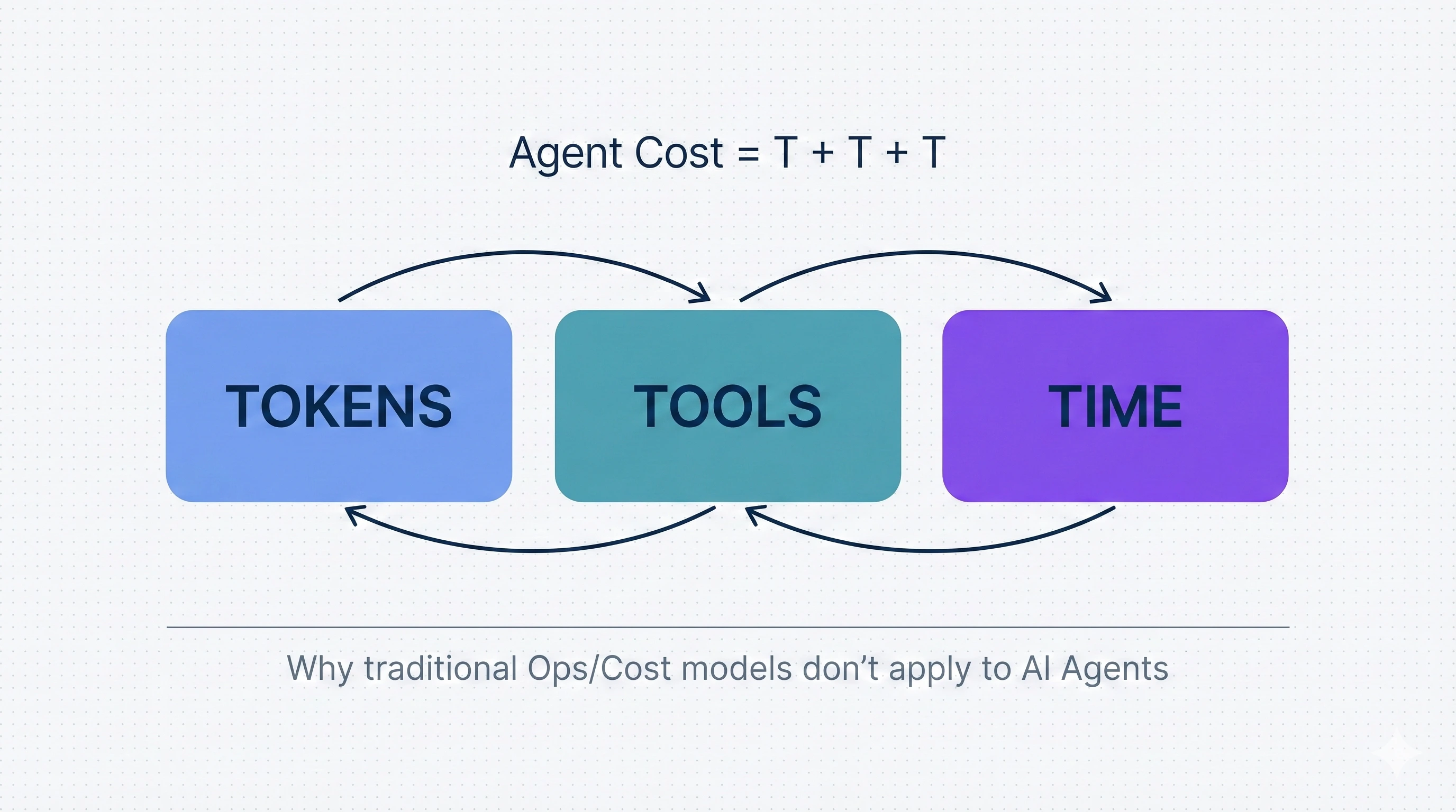
2. Agent Cost = Tokens + Tools + Time (TTT)
TTT is like a “cost conservation law” for Agents. Similar to the CAP theorem in distributed systems, you always trade off 2 out of the 3 parameters.
2.1 Tokens
This is usually the largest cost. An Agent does not just “respond”. It thinks.
Tokens are charged for three things:
- Reasoning: Internal reasoning steps (chain-of-thought, planning loops). The user does not see them, but you still pay for them.
- Context Inflation: The longer the session, the bigger the prompt. The 10th request is more expensive than the 1st one.
- Guardrails & Eval: Secondary models running in parallel for moderation, policy checks, and scoring.
2.2 Tools
An Agent does not handle everything by itself. It interacts with external systems.
API Fan-out
A simple request like “Check order status” may call:
- CRM
- Shipping
- Inventory
- Refund policy
- Billing
3–5 tool calls per request is very normal.
Egress & External API
When the Agent orchestrates workflows, it generates additional API usage fees and network costs.
2.3 Time
If Tokens are the cost of “thinking”, then Time is the cost of “existing”. You pay for infrastructure:
- vCPU
- RAM
- Instance hours
- Idle time (waiting for LLM/tool responses while the instance is still running)
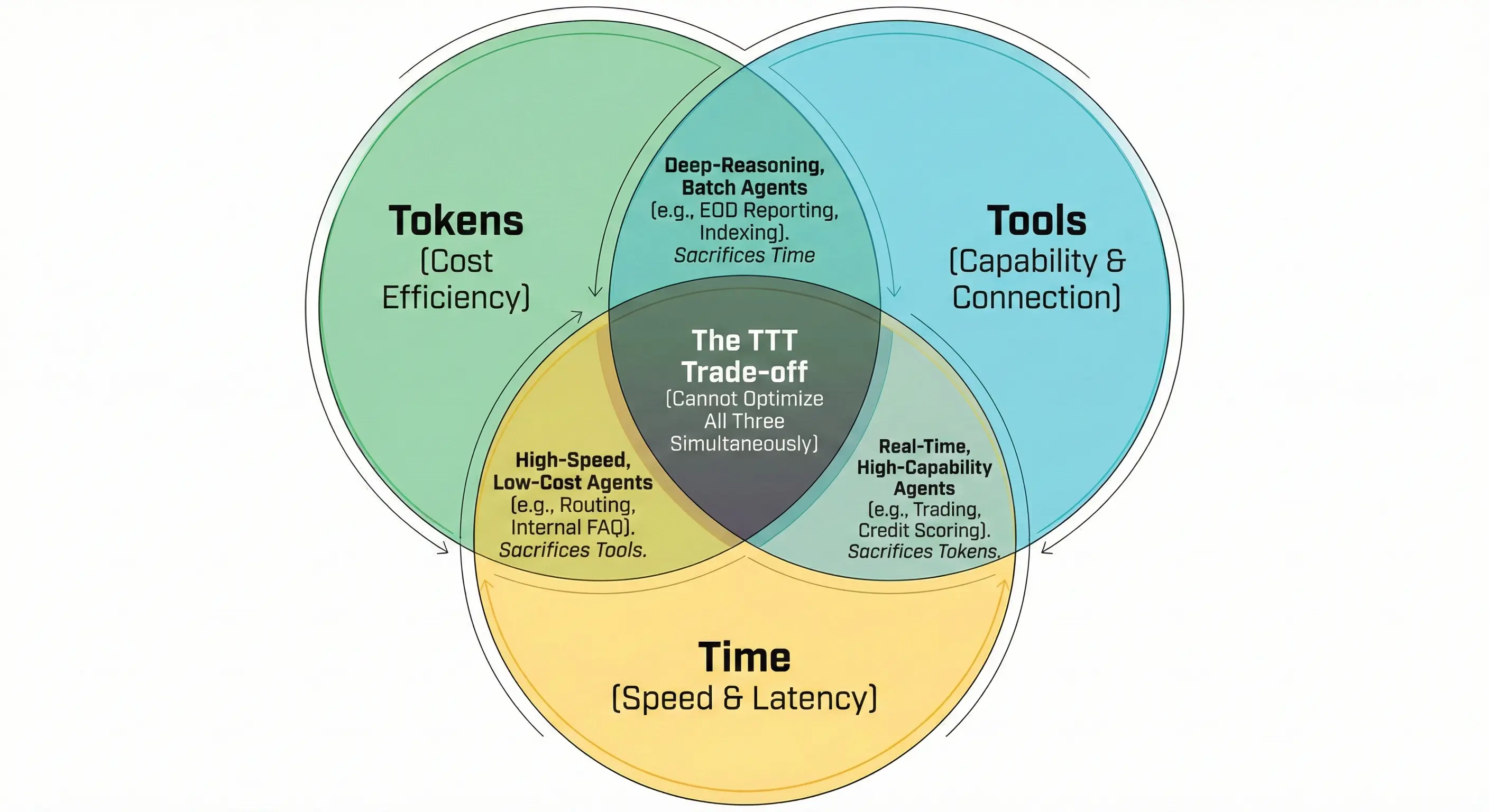
Similar to the CAP theorem, you cannot optimize Time, Token, and Tool at the same time. Every decision that optimizes one parameter will impact the other two.
Depending on the business problem, you need to decide which parameter is your competitive advantage:
- Faster (optimize Time)
- Cheaper (optimize Token)
- More powerful (optimize Tool capability)
From there, design the system intentionally to control the remaining two. Because cost never disappears. It only shifts from one form to another.
3. Pricing Models
After understanding how TTT works, the next important question is not how much it costs, but how to price it in a way that reflects the true nature of an Agent. Below are the three most common approaches.
3.1 – Per-request (Unit Economics)
The question:
How much does one request cost?
This is unit cost — measuring how much a single request costs.
Token Cost
Unlike a normal LLM call (Input → Output), an Agent runs in loops. The formula is:
\[C_{token} = \sum_{step=1}^{k} \left( T_{in, step} \times P_{in} + T_{out, step} \times P_{out} \right)\]Where:
- k: Number of reasoning steps (iterations) to finish the task.
- T_in: Total input tokens at each step (including System Prompt, Tool Definition, conversation history, and tool results from the previous step).
- T_out: Output tokens at each step (including Reasoning/Chain of Thought and tool call instructions).
- P_in: Cost per input token (for example: $2 / 1M input tokens).
- P_out: Cost per output token (for example: $10 / 1M output tokens).
Tool Cost
\[C_{tools} = \sum_{i=1}^{n} (P_{ext,i} + P_{token,i} + P_{infra,i})\]Where:
- n: Average number of tool calls to complete a task (for example: 1 user request → 3 tool calls).
- P_ext: Direct fee from the external API provider (for example: $0.001 per call).
- P_token: Token cost for the LLM to process the tool interaction.
- P_infra: Egress bandwidth or intermediate compute cost between Agent and Tool.
Time Cost
\[C_{time} = (vCPU \cdot L + GiB \cdot L) \cdot \$_{infra}\]Where L is the actual processing time (for example: 0.004 hour, since most cloud infra is billed per hour, e.g., $4/hour).
Purpose: Calculate how much one request costs at runtime. This is useful to prove optimization methods (prompt optimization, caching, async tools, model tuning).
- Reduce 20% tokens → directly reduce cost per session.
- Reduce tool calls from 5 to 2 → reduce cost.
- Caching → reduce both Token and Time cost.
3.2 – Concurrency / Sessions
The question:
How many active users at peak?
Here, Tokens and Tools are not just money — they are quota and rate limits.
Concurrency measures how many users are interacting with the system at the same time during peak hours.
This model ignores individual requests and focuses on the maximum concurrent users the system must support, to ensure the Agent does not fail during peak time.
Purpose:
Measure how much capacity is needed at peak to protect p95 latency. Used to set max_instances.
Token Cost
\[TPM_{required} = \frac{Peak\_C \cdot T_{total\_per\_session}}{Duration_{session}}\](TPM: Tokens Per Minute — the model provider’s bandwidth limit, meaning how many tokens can pass through the system per minute.)
Tool Cost
\[RPM_{tool} = Peak\_C \cdot n \cdot P_{buffer}\](RPM: Requests Per Minute — backend/API system rate limit.)
Time Cost
\[C_{peak} = Peak\_C \cdot (vCPU_{sess} + RAM_{sess}) \cdot H_{peak}\](Where Peak_C is Peak Concurrent Sessions.)
Emerging Problems
1. Token Rate Limit (TPM/RPM)
If 100 sessions run at the same time and each burns 2,000 tokens:
- Does the API have enough TPM?
- If it exceeds the limit → 429 errors → the Agent cannot respond.
2. Tool Backend Capacity
100 users call CRM at the same time:
- Can the current backend handle it?
- Retry → session stays longer → increase Time cost.
In this model:
- Tokens = quota pressure
- Tools = backend stress
- Time = compute capacity
3.3 – Shape / Window
In the Shape / Window model, we do not calculate “how much one request costs”. Instead, we look at the total system resource usage and the real operating time window (peak hours, daily, monthly) to align directly with Cloud Provider or SaaS invoices.
This shifts the thinking from cost per request to cost by footprint and cycle, because providers charge by load, time, and total volume — not by individual requests.
Token Cost
\[C_{total\_token} = \sum (Tokens_{Realtime} \times P_{standard}) + \sum (Tokens_{Batch} \times P_{discount})\]With condition:
\[Max(Tokens_{Realtime} / Minute) \leq Shape_{TPM}\]Similar to electricity pricing, Token cost also has the concept of Window (time window) , enabled by features like Batch APIs.
- Peak Window: Real-time Agent requests must accept 100% listed price.
- Off-Peak Window: Non-urgent Agent tasks (like end-of-day report scanning, data aggregation, RAG indexing) can be pushed into Batch Window (often 24h).
Tool Cost
\[C_{tool} = \sum (Calls_{total} \cdot P_{tool})\]Time Cost
\[C_{time} = (Inst_{peak} \cdot H_{peak} + Inst_{off} \cdot H_{off}) \cdot P_{instance\_hour}\]Where:
- Inst: Number of deployed servers/containers.
- H: Running hours (split by Peak / Off-peak).
- P: Unit price (Token, vCPU, Tool call).
4. Conclusion
Managing cost for AI Agents is not about counting every single token. It is about understanding the nature of the problem and choosing the right measurement model.
The pricing approach depends on the goal and the stage of the system:
- Unit Economics (Per-request): Used during R&D and Optimization. This method helps Devs and SAs measure the impact of prompt optimization, redesigning reasoning loops, or replacing one model with another — and see how those changes affect both cost and output quality.
- Concurrency / Sessions: Used for Sizing & Capacity Planning. This is the protection layer before going to production: define max instances, set rate limits (TPM/RPM), and make sure the system does not crash when traffic spikes.
- Shape / Window: A tool for Financial Management and FinOps. This approach connects the technical system with the real invoice from the Cloud Provider. It optimizes cash flow based on operating cycles instead of individual requests.
Best practices for Costing & Sizing design:
- Make SLA the center: With the TTT trade-off, you cannot optimize all three at the same time. For core systems that require high accuracy, security, and reliability (for example: investment advisory, document assessment, or transaction processing), prioritize investment in Tools (strong Guardrails, high-accuracy RAG layers) and Time (reserved infrastructure for peak hours). Accept higher Token cost in reasoning flows to gain safety and correctness.
- Route workloads by urgency (Routing by Urgency): Fully leverage the Shape/Window model. Clearly separate real-time tasks (like live advisory) from tasks that can wait (end-of-day report scanning, data aggregation, RAG indexing). Push as many background tasks as possible into off-peak windows or Batch APIs.
- Design Circuit Breakers from day one: When sizing the system, the biggest risk is not the number of users — it is an Agent stuck in an infinite loop or retrying a failing API endlessly. Always implement timeout mechanisms, max reasoning iterations, and max tool calls per session to protect the system’s TPM/RPM quota from being exhausted.